Lidar SLAM

LOAM

LOAM

• LOAM use a new defined feature system (corner and flat point), for the detail see its article.
• LOAM suppose linear motion within the scan swap (VLOAM further uses visual odometry to estimate it), and undistort the lidar points.
• LOAM has a low frequence optimization thread.

A-LOAM

• LOAM has IMU refinement.
• Lack feature filter in A-LOAM.
• LOAM implies the LM solver itself. A-LOAM uses Ceres solver.
• LOAM use analytical derivatives for Jacobians, but A-LOAM uses the automatic derivatives offered by Ceres (which is exact solution but a little bit slower).

Performance:

• A-LOAM seems good,less redundant points.
• but has more error in far edges.
• LOAM method has no assumption of a consistent “floor”, that is better for our case.
• A-LOAM has the same logical with LOAM, but its performance is much worse.

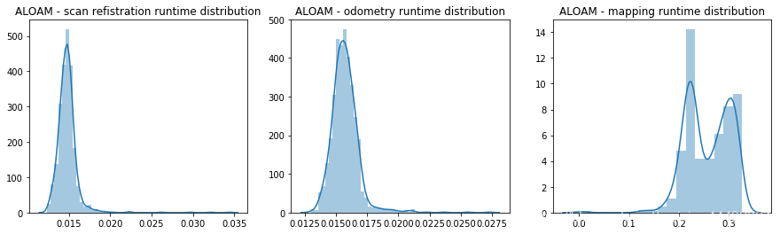
• ALOAM - scan refistration the maximum time is : 0.034434 the mean of time is : 0.0148146394612
• ALOAM - odometry the maximum time is : 0.027296 the mean of time is : 0.0157431030928
• ALOAM - mapping the maximum time is : 0.326849 the mean of time is : 0.257764385093

LeGO LOAM

vs LOAM:

• Faster and similar accuracy as LOAM, and has a better global map visual effect.

Difference LOAM:

• Add segmentation before processing (gound extraction and image-based segmentation)
• Sub-divide the range image before feature extraction → more evenly distributed features.
• Label match
• Two step LM. Seperate the optimization based on different property of edge and planar points. Becomes faster while similar accuracy.
• Difference map storage method, can use pose graph optimization and use loop closure.

Performance:

• lego slam has the best result, error is small.
• Flat plane has good look, achieve a dense map, while keep its consistence.

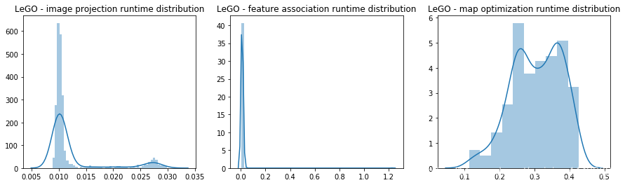
• LEGO LOAM - image projection the maximum time is : 0.029819 the mean of time is : 0.0123906096595
• LEGO LOAM - feature association the maximum time is : 1.226773 the mean of time is : 0.0126770831335
• LEGO LOAM - map optimization the maximum time is : 0.427468 the mean of time is : 0.30585172524

For one input scan, it takes 0.0249s in average. It is about 25% faster than ALOAM.

HDL-GRAPH-SLAM

• It is basically a graph optimization algorithm.
• Use ICP-based or NDT-based methods to register new point cloud, and match candidates of loop closure.
• Assumed a shared ground plane.
• For the graph optimization part, it use the most sample edge for consecutive frames, along with the floor observation edge.
• Too simple loop closure processing.
• In summary, it uses the most basic algorithms, however it has a complete structure.

Performance:

• not that much error for the far points, as it has loop closure
• lots of redundant points as it has no optimization on point cloud, floors and walls are very thick in the global map.

• HDL - prefiltering the maximum time is : 0.395365 the mean of time is : 0.00943357786885
• HDL - floor detection the maximum time is : 0.856617 the mean of time is : 0.0456638586777
• HDL - odometry the maximum time is : 0.309964 the mean of time is : 0.0742533234078
• HDL - graph slam the maximum time is : 2.140327 the mean of time is : 0.13695704878

Its processing time is much more than the other two methods, as it use NDT, while the other use feature points.

IMLS-SLAM

Implicit Moving Least Squares(IMLS) surface represetation is used to handle large amount and sparisty of acquired data. It makes me proud to see some schoolmates made such a contributional work. paper

Pretreatment

1. Unwarp lidar scan, It is done b linear interploation using the last relative pose.

\[\bar{\tau}(t_{k}) = \tau(t_{k-1}) * \tau(t_{k-2})^{-1} * \tau(t_{k-1})\]

\[\tau(t) = Interpolation(\bar{\tau}(t_{k}), \tau(t_{k-1}), t), t \subseteq (t_{k-1}, t_{k})\]

2. remove small size segmented point cloud, and grouped cloud with small bounding box.

Scan sampling

• Classic ICP uses random sampling method, this may fail in many cases.
• A selected suitable sampling method was proposed to improve ICP. But computational expensive.
• This article proposed a sampling method based on the observability of the point of different angle and of the unkown translations. To choose better and fewer points for matching.

Scan-Model Match

• Kinect fusion uses TSDF for scan-to-model match, but TSDF surface is defined by a voxel grid (empty . SDF, known) and then is usable only in a small volume space. As a result, TSDF cannot be used in large outdoor environment.
• This article uses IMLS (Implicit Moving Least Square) surface (the set of zeros of a function)

VIL-SLAM

It is a Stereo Visiual Inertial Lidar SLAM. Compared to VLOAM, this work uses a tightly coupled VIO (VLOAM uses a loosely coupled one), and VIL-SLAM has a Lidar enhanced loop closure. paper

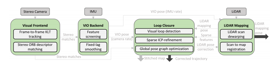
1. Stereo visual KLT optical flow tracking and ORB feature matching.
2. IMU preintegartion, and tightly coupled VIO (until this part, it is tha same as VINS-Fusion).
3. Use the VIO output pose to unwarp the lidar scan. And registre the scan by Edge and planar points (LOAM method)

4. Loop clousre.

   1. Propose candidates by Bag-of-Words.
   2. PnP(Perspective-n-Point) to obtain relative pose initial estimation (of VIO).
   3. Use ICP to refine the estimation (of Lidar Odometry).

In my point of view, this work is a mixture of a tightly coupled VIO (VINS) and a loosely coupled Lidar Visual (VLOAM). Can be seen as a update version of V-LOAM.